
[mathjax]
Some math is necessary to get started with machine learning and understand most of the beginner discourse on the topic, especially if you are looking into the theory of it. So let’s get you started with some of the basic terminology and objects that are important from the area of linear algebra.
Why do we need Linear Algebra for Machine Learning?
If you are already convinced that you need Linear Algebra, you can skip this part. If not, let’s talk about neural networks for a second.
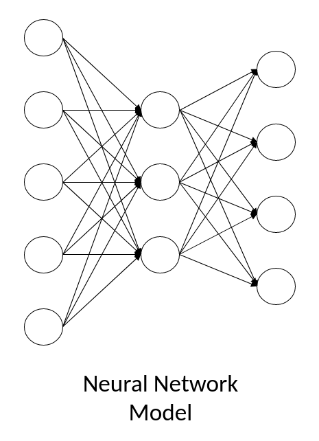
Often you see models presented like this.
But really, once we think about the data, we should visualize a neural net more like this:

The left block is the input data that gets transformed step by step.
The weight layers previously depicted by crossed lines are now red lines, where the data is changed through a linear transformation each by multiplying a matrix of weights with the incoming data, which results in data with different contents and possibly a different shape. In addition, neural networks add a non-linear “activation” function, however that is not the focus of this example.
You can see how we have a matrix of data (explained below) at each step and even the linear transformations in between the steps are operations of the world of linear algebra and as such neural networks and other areas of machine learning are closely related to linear algebra. In most machine learning methods, you have a table of data points as input and they need to be used and transformed for which linear algebra is a natural tool.
So let’s look at some common objects within linear algebra:
Scalars
Scalar is the math-word for a single number. Variables that are scalars are written as lower case, for example $\text{let } s \in \mathbb{R}$ would define $s$ to be a real number like $3.145$ or $1/3$ or simply $2$.
Vectors
Vectors are arrays or lists of numbers – well technically arrays of any type of data, but in the Machine Learning context they are generally filled with numbers.
You define them like this: $\text{let } x \in \mathbb{R}^n$ and then $x$ (again, typically lower case) is a vector of length $n$. If you want to show its entries as, you can write it as in the following image where you can also see that the individual entries are called $x_1$, $x_2$ and so on.

Notice how the indexing starts at $1$ in math, unlike in programming where we typically start counting at 0.

As a mental guide you can envision a vector (especially a vector with 2 or 3 entries) as a point in space or as the arrow from the origin towards that point in space. That mental picture falls apart quite easily in higher dimensions as is common in math, but it might still help.
Matrices
Matrices are two-dimensional arrays of numbers or you can envision them as a table of numbers.
You define one like this: $A \in \mathbb{R}^{m \times n}$, when it has $m$ rows and $n$ columns.

To index or address single entries within the matrix you use subscripts similar to vector entries, but with two dimensions. For example $A_{1,1}$ is the top left corner – the entry in the first row and first column. The one next to it to the right would be $A_{1,2}$ – first row, second column. And the lower right entry is $A_{m, n}$ – $m$th row, $n$th column. Remember: in math you start counting at 1, not at 0 like in coding.
Tensors
Tensors sound complicated but really they are just matrices with more than 2 axes. For example the following image shows how you would define a three-dimensional tensor:

These are not common in mathematics, but very common in machine learning, specifically deep learning. Why is that?

Take of example a dataset that consists of images. Images by themselves are already two-dimensional: they consist of pixels that are ordered within the width and height of the picture. But the input of a neural network is often a stack of data, in this case a stack of images, because that allows the GPU to use its parallel computing to process multiple images at the same time which speeds up the training of the predictive model.
And a stack of images is three-dimensional: two dimensions for the images themselves and the third dimension is the height of the stack if you imagine the images printed out and stacked on top of each other. Which is why you often encounter tensors in machine learning.
Transpose
Next up are some common operations on these objects we just looked at. The first of these is the matrix transpose.
Transposing basically just means mirroring. Imagine laying a mirror along the main diagonal of the matrix as indicated in the image below. The diagonal underneath the mirror stays the same, but everything from the upper right triangle goes to the lower left and the reverse is also true.
You can also imagine writing each row of the original matrix as a column in the transposed matrix. Instead of writing from left to right, you write each row from top to bottom.

The transpose also applies to vectors. In this case it just transforms a column vector into a row vector and vise-versa.

Addition
Matrix addition is fairly straightforward. You simply add each entry to the entry in the same position in the other matrix. However, this is only allowed or defined if the matrices have the same shape, that is the same number of rows and columns.

Below you can see an example. we add the $2$ and $0$ in the upper left corner, the $1$ and $3$ from the upper right corners and so on.

Scalar Multiplication
You can also multiply a matrix with a number – which is called a scalar as you have seen above. This simply works element-wise, the number will be multiplied with each entry in the matrix at the respective position as you can see in the example below.

Broadcasting
This technique is not really something that exists in linear algebra, but it is very much used as a simplified notation in coding languages like Python.
The general idea is that the smaller matrix will be extended by copies of itself to fit the bigger matrix to make things like matrix addition possible even if the matrices don’t have the same dimensions.
Below you can se an example of a scalar added to a matrix. What implicitly happens under the hood of the programming language is that the 2 is extended to a matrix with two rows and two columns to match the bigger matrix and each entry of this new matrix will be 2. Then the addition is possible like below.

Here is another example of column vector being added to a 2×2 matrix. In this case the column will be duplicated, because the row dimension already matches the matrix, but the columns did not match before. After duplicating the column next to itself, the matrix has the correct format for addition and you can see what will be calculated in this case.

Sources and further reading
Most of this knowledge comes from studying linear algebra and using Python for a while, however if you want to read about this in more detail, I can recommend the chapter Linear Algebra from the Deep Learning Book. Freely available online and in general a fantastic resource 🙂